| Version 2 (modified by , 16 years ago) (diff) |
|---|
Package BysPrior
BysPriorInf stands for Bayesian Prior Information and allows to define prior information handlers to be used in estimation systems (max-likelihood and bayesian ones).
A prior is a distribution function over a subset of the total set of variables of a model that expresses the knowledge about the phenomena behind the model.
The effect of a prior is to add the logarithm of its likelihood to the logarithm of the likelihood of the global model. So it can be two or more priors over some variables. For example, in order to stablish a truncated normal we can define a uniform over the feasible region and an unconstrainined normal.
In order to be estimated with NonLinGloOpt (max-likelihood) and BysSampler (Bayesian sampler), each prior must define methods to calculate the logarithm of the likelihood (except an additive constant), its gradient and its hessian, and an optional set of constraining inequations, in order to define the feasible region. Each inequation can be linear or not and the gradient must be also calculated. Note that this implies that priors should be continuous and two times differentiable and restrictions must be continuous and differerentiable, but this an admisible restricion in almost all cases.
Chained priors
A prior can depend on a set of parameters that can be defined as constant values or another subset of the model variables. For example we can define hierarquical structures among the variables using a latent variable that is the average of a normal prior for a subset of variables. We also can consider that the varianze of these normal prior is another variable and to define an inverse chi-square prior over this one.
Non informative priors
Let  a uniform random variable in a region
 which likelihood function is

Since the logarithm of the likelihood but a constant is zero, when log-likelihood is not defined for a prior, the default assumed will be the uniform distribution, also called non informative prior.
Domain prior
The easiest way, but one of the most important, to define non informative prior information is to stablish a domain interval for one or more variables.
In this cases, you mustn't to define the log-logarithm nor the constraining
inequation functions, but simply it's needed to fix the lower and upper
bounds:

Polytope prior
A polytope is defined by a system of arbitrary linear inequalities

We can define this type of prior bye means of a set of  inequations due NonLinGloOpt doesn't have any special behaviour for linear
inequations, and it could be an inefficient implementation.
inequations due NonLinGloOpt doesn't have any special behaviour for linear
inequations, and it could be an inefficient implementation.
However we can define just one non linear inequation that is equivalent to the full set of linear inequations. If we define

then
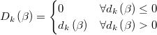
is a continuous function in  and
and
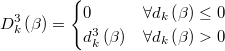
is a continuous and differentiable in 
The feasibility condition can then be defined as a single continuous nonlinear inequality and twice differentiable everywhere
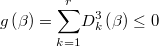
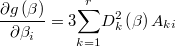
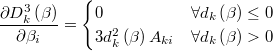
The gradient of this function is