| Version 22 (modified by , 15 years ago) (diff) |
|---|
Package QltvRespModel
Max-likelihood and bayesian estimation of qualitative response models.
Weighted Boolean Regresions
Abstract class
@WgtBoolReg
is the base to inherit weighted boolean regressions as logit or probit or any other,
given just the scalar distribution function  and the
corresponding density function
and the
corresponding density function  . In a weighted regression
each row of input data has a distinct weight in the likelihood function. For
example, it can be very usefull to handle with data extrated from an stratified
sample.
. In a weighted regression
each row of input data has a distinct weight in the likelihood function. For
example, it can be very usefull to handle with data extrated from an stratified
sample.
This class implements max-likelihood estimation by means of package NonLinGloOpt and bayesian simulation using BysSampler.
Let be
 the regression input matrix
 the vector of weights of each register
 the regression output matrix
The hypotesis is that 
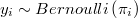
![\pi_{i}=Pr\left[y_{i}=1\right] = F\left(X_{i}\beta\right)](../chrome/site/images/latex/838c94f04418fa55336d6713bf038357.png)
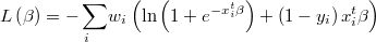
The likelihood function is then
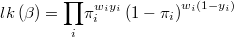
and its logarithm

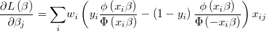
The gradient of the logarithm of the likelihood function will be
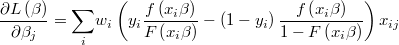
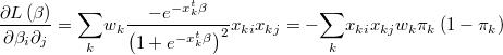
and the hessian is

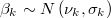
User can and should define scalar truncated normal or uniform prior information and
bounds for all variables for which he/she has robust knowledge.

When  is infinite or unknown we will express a uniform
prior.
When
is infinite or unknown we will express a uniform
prior.
When  or unknown we will express that variable
has no lower bound.
When
or unknown we will express that variable
has no lower bound.
When  or unknown we will express that variable
has no upper bound.
or unknown we will express that variable
has no upper bound.
It's also allowed to give any set of constraining linear inequations if they
are compatible with lower and upper bounds

Weighted Logit Regression
Class @WgtLogit is an specialization of class @WgtBoolReg that handles with weighted logit regressions.
In this case we have that scalar distribution is the logistic one.
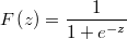
Scalar cumulant:
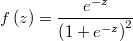
Scalar density:
Scalar density derivative:

Logarithm of likelihood:
Gradient:

Hessian:
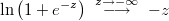
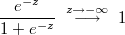
From the standpoint of arithmetic discrete numerical calculation must take into account that

For this reason we must carefully try to contain the exponential expressions.
In this case it will use the following asymptotic equalities
Weighted Probit Regression
Class @WgtProbit is an specialization of class @WgtBoolReg that handles with weighted probit regressions.
In this case we have that scalar distribution is the standard normal one.
Scalar cumulant:

Scalar density:

Scalar density derivative:
Logarithm of likelihood:

Gradient:
Hessian:

To avoid numerical problems will use the following equality
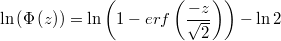
The function logarithm of complemetary error function
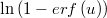
is implemented as gsl_sf_log_erfc that is available in TOL.
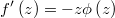
In the gradient it appears two times the Hazard function
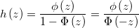
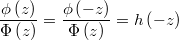
decreases rapidly as  approaches
  and asymptotes to
 as approaches
Hazard function is implemented as gsl_sf_hazard that is also available in TOL.